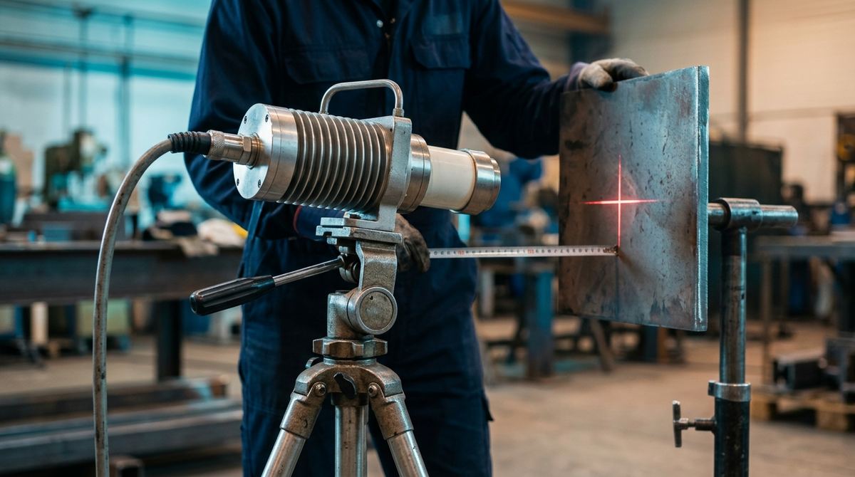
Two radiographic systems with the same maximum voltage can produce images of very different quality. The difference almost never lies in the number on the nameplate, but in less advertised quantities: the focal spot, the exposure geometry, the high-voltage waveform, the filtration, the thermal capacity of the anode. This article lines up the physics that actually matters at work — with formulas, numbers and worked cases — and is the applied companion to our purchasing guide how to choose an industrial X-ray tube and generator: there the commercial selection criteria, here the physical why behind each parameter. The industry's reference terminology is codified in ISO 5576, the vocabulary of industrial radiology.
Focal spot and geometric unsharpness: the foundation of everything
The beam is not born from a point: it is born from an area of the anode, the focal spot, whose projection along the beam direction is the effective focal spot (the anode angle makes it smaller than the area actually bombarded). Because the source is extended, every edge of the part projects a blurred transition zone onto the image: the geometric unsharpness Ug. The formula is elementary:
Ug = f · b / a, where f is the focal spot size, a the source-to-object distance (SOD) and b the object-to-detector distance (SDD − SOD). In equivalent form: Ug = f · (SDD − SOD) / SOD.
Worked case: a tube with a 2.0 mm focal spot, part 600 mm from the source, detector at 660 mm (b = 60 mm): Ug = 2.0 × 60 / 600 = 0.2 mm. If the same part is radiographed at SOD = 300 mm with the detector still 60 mm behind it, the unsharpness doubles to 0.4 mm: fine details (small pores, the thin IQI wires) start to smear. This is why ISO 17636 imposes minimum source-to-object distances through nomograms as a function of focal spot, thickness and technique class (class B is more demanding than class A): geometry is not an aesthetic preference, it is a normative requirement.
Beware of nameplate values: the "nominal focus" and the measured focal spot do not necessarily coincide. For industrial X-ray systems the measurement is standardized by the EN 12543 series (parts 1–5), which defines the methods — scanning, pinhole camera, slit camera, edge method — and, in part 5, the measurement of the effective focal spot of mini and microfocus tubes; in the medical field the corresponding convention is IEC 60336. When comparing two tubes, always ask by which method the spot is declared: two "1 mm" spots measured with different methods are not the same tube.
Minifocus and microfocus: geometric magnification
Shrinking the focal spot does more than contain unsharpness: it lets you put geometry to work for you, with projective geometric magnification. Moving the part closer to the source magnifies the image by a factor M = SDD / SOD, and the unsharpness referred to the part is f · (M − 1) / M — but the most direct way to reason is at the detector plane: Ug = f · (M − 1).
Worked case (electronics / additive manufacturing): a microfocus with f = 5 µm, part at SOD = 30 mm, detector at SDD = 300 mm: M = 10, Ug = 5 × 9 = 45 µm at the detector plane. With a 100 µm pixel detector, the pixel referred to the part is 100/10 = 10 µm: you resolve voids in BGA solder joints, bonding wires, internal channels of a 3D-printed component. The same magnification with a conventional 1 mm spot would give Ug = 9 mm: an unusable image. It is this spot-magnification combination, not the detector alone, that decides the system's real resolution; the flip side is flux: in microfocus tubes power is measured in watts, not kilowatts, and times stretch. On the opposite front, for panel selection and its parameters see how to choose a DR detector, and for high-resolution volumetric imaging our guide to industrial CT scanning.
kV: energy, contrast, thickness
The anode voltage sets the maximum photon energy and hence penetration capability, but also contrast: at lower energies photoelectric absorption dominates, strongly dependent on thickness and atomic number, so thickness differences translate into strong density differences; at higher energies Compton scattering dominates and the image flattens. Hence the practical rule: the lowest kV compatible with the penetrated thickness and with reasonable times. ISO 17636 publishes maximum allowed voltage curves as a function of thickness and material: they are a normative ceiling, not the working value.
Worked case (steel vs aluminium): a steel joint with 20 mm penetrated thickness is typically worked in the 160–220 kV band, with exposures of a few minutes on film and much shorter on DR; a 40 mm aluminium casting, although thicker, is radiographed at far lower voltages (indicatively 80–120 kV), because aluminium's atomic number and density are a fraction of iron's. Using 220 kV on aluminium "because the tube has them" produces a flat image in which fine shrinkage porosity disappears. The everyday operational tool is the set of exposure charts for your own system: kV / thickness / mA·min diagrams built for your tube, your distance and your detector, to be rebuilt whenever any of those changes.
mA·s, reciprocity and filtration
At a given kV, the quantity of radiation is proportional to the product current × time (mA·s or mA·min): within broad limits, 5 mA for 2 minutes equals 10 mA for 1 minute, and the choice is driven by the tube's thermal capacity and by site constraints. Additional filtration (copper or aluminium sheets at the window) removes the soft tail of the spectrum: low-energy photons that would not cross the part anyway but generate scatter and fog. The "hardened" beam improves the contrast-to-fog ratio on medium-to-heavy sections and is often required by procedures; the trade-off is a small increase in exposure time. On the detector side, the complement is lead screens (film) and backscatter control.
| Parameter | Main effect | Practical rule |
|---|---|---|
| Focal spot (f) | Sharpness: unsharpness Ug = f·b/a | Small for detail; large for power and short times |
| SOD / SDD | Unsharpness and magnification M = SDD/SOD | Respect ISO 17636 minimum distances; magnify only with small spots |
| Voltage (kV) | Penetration and contrast (inverse) | The lowest practicable kV; maximum-voltage curves as a ceiling |
| Current × time (mA·s) | Quantity of radiation, density/SNR | From the exposure charts; reciprocity within thermal limits |
| Filtration (Cu/Al) | Beam hardening, less scatter fog | On medium-to-heavy sections and where the procedure requires it |
| Waveform (CP vs unipolar) | Effective flux and spectrum stability | CP for productivity and repeatability; unipolar where weight and cost matter |
Site case: a portable tube on a pipeline
Third case, the harshest: radiography of girth welds on site, dozens of welds per day, generator power, wide temperature swings. Here the less flashy nameplate parameters come into play:
- Duty cycle and cooling: the beam energy is a tiny fraction of the electrical power: almost all of it becomes heat in the anode. Gas- or forced-air-cooled portable tubes declare their duty cycles: some run continuously at reduced current, others require intermittent cycles (for example pauses comparable to the exposure times at maximum ratings). Over 40 joints/day, the difference between a continuous duty cycle and a 50% one is an hour or more of cumulative waiting.
- Constant potential vs unipolar: constant-potential (CP) generators keep the high voltage stable: the whole exposure time works at full energy, with a repeatable spectrum and shorter times at the same nominal kV. Unipolar/pulsed circuits are simpler and lighter, but part of the cycle produces reduced-energy photons: longer, less repeatable exposures. On site the choice is a trade-off between productivity and the weight carried on your shoulder.
- Directional or panoramic: a panoramic tube emits over 360° perpendicular to its axis: positioned at the pipe centre with a crawler, it exposes the entire joint in a single single-wall exposure, replacing the three or more double-wall exposures of a directional tube. On pipelines it is the single largest productivity multiplier; exposure geometries and the typical joint defects are covered in the twin article radiography of welds and castings: applied cases.
- Radiation safety: in Italy the use of X-ray generators is a practice subject to Legislative Decree 101/2020: oversight by a qualified radiation protection expert, controlled areas, training. On site, beam geometry (collimation, direction) is also a radiation-safety tool, not only an image-quality one.
From parameters to instrument: the next step
Translating these numbers into a concrete configuration — maximum voltage, focal spot or spots, waveform, cooling, directional or panoramic, and the detector to pair — depends on your materials, thicknesses and volumes. PITECH supports Italian industry in specifying and supplying industrial radiography systems, from generator to detector, with application evaluations on the customer's real samples: describe your application via the contact page, by form, WhatsApp or email.
Frequently asked questions about X-ray tubes and parameters
What is the focal spot of an X-ray tube?
It is the area of the anode from which the X-ray beam is emitted, seen from the direction of the emerging beam (effective focal spot). The smaller it is, the sharper the image, because geometric unsharpness shrinks; the larger it is, the more thermal power it can sustain, hence more flux and shorter exposure times. The nominal value declared by the manufacturer must be read against the standardized measurement methods, such as the EN 12543 series for industrial X-ray systems.
How is geometric unsharpness calculated in radiography?
With the formula Ug = f × b / a, where f is the focal spot size, a the source-to-object distance and b the object-to-detector distance. It is equivalent to Ug = f × (SDD − SOD) / SOD. Example: a 2 mm focal spot, object 600 mm from the source, detector at 660 mm: Ug = 2 × 60 / 600 = 0.2 mm. To reduce it, increase the source-to-object distance, bring the detector closer to the part, or use a smaller focal spot.
Is higher or lower kV better in industrial radiography?
The lowest kV compatible with the thickness to be penetrated and with reasonable exposure times: lower voltages give more contrast, higher voltages give more penetration and latitude but flatter images. ISO 17636 publishes maximum-allowed-voltage curves as a function of thickness and material: they are a ceiling, not a recommended working value. For the same thickness, aluminium requires far lower voltages than steel.
What is the difference between a minifocus and a microfocus tube?
Orders of magnitude of the focal spot: a conventional tube typically sits between 0.5 and a few millimetres, a minifocus between a few tenths of a millimetre and ~50 micrometres, a microfocus below 50 micrometres, down to a few micrometres. A small spot enables projective geometric magnification (M = SDD/SOD) without losing sharpness: this is what makes inspection of electronics, micro-welds and additive-manufactured parts possible; the price is much lower flux and therefore longer times.
When is a panoramic X-ray tube needed?
When complete circular joints must be radiographed in a single exposure: a panoramic tube emits its beam over 360 degrees perpendicular to the axis and, positioned at the centre of a pipe or vessel (for example with a crawler in pipelines), exposes the whole circumference in one shot with single-wall geometry. It replaces the 3 or more exposures of the double-wall technique, with a very large productivity gain on pipeline sites.