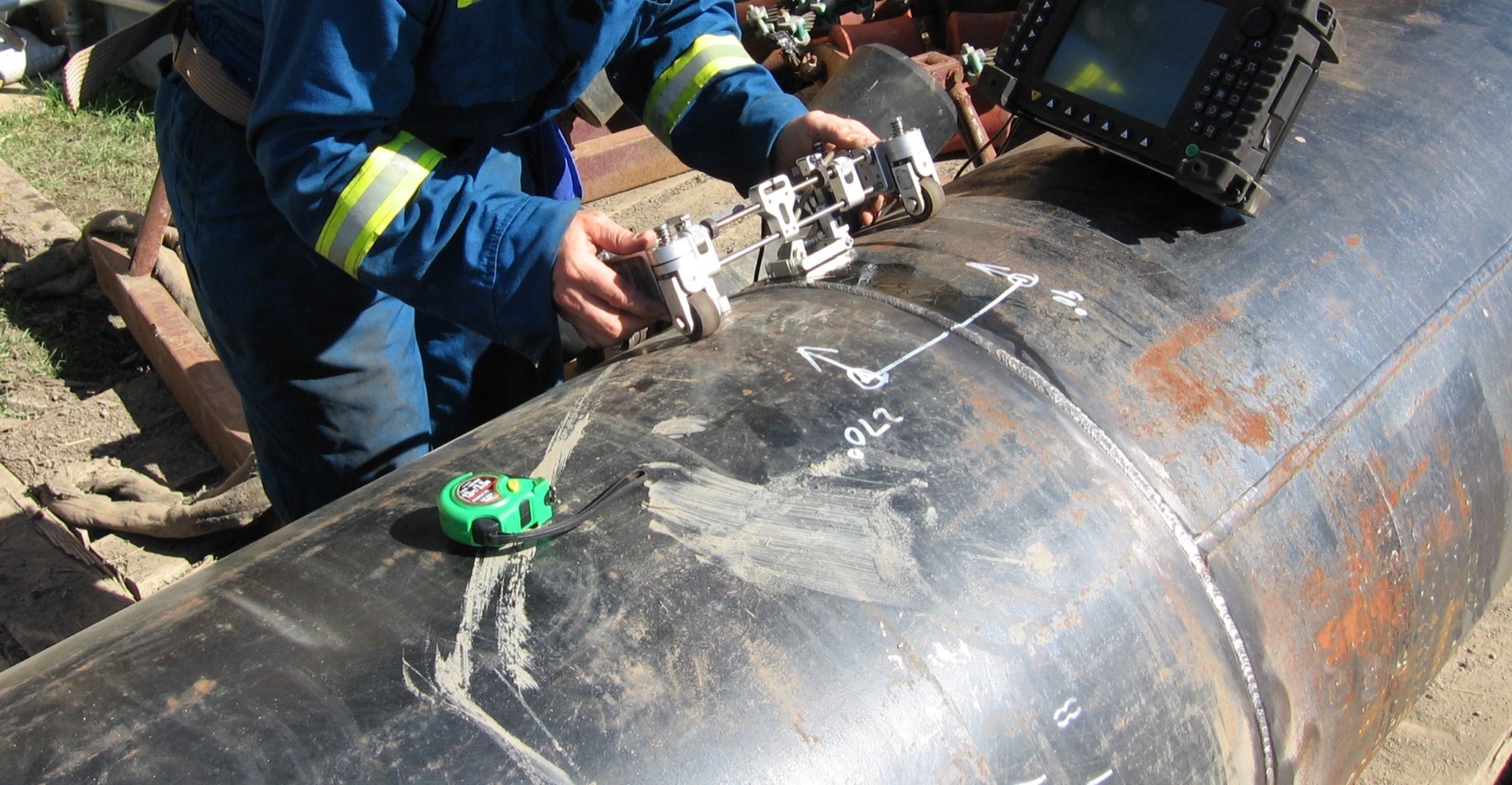
In the maintenance of oil & gas, chemical, power and marine assets, most recurring NDT work is not about finding manufacturing defects: it is wall loss monitoring. Internal corrosion, erosion, corrosion under insulation, localised attack downstream of an injection point — all of these reduce to a single measurable parameter, the remaining wall thickness. The ultrasonic thickness gauge measures it from one side only, in seconds, without shutting down the asset and without removing material.
Getting a number is the easy part: any instrument will produce one. The hard part — the difference between a useful inspection and a list of figures — is getting a number that is correct, repeatable and comparable over time, because the engineering value does not lie in the single reading but in the historical series from which corrosion rate and remaining life are calculated. This guide goes into the substance: physics, measurement modes, systematic errors, selection criteria and how the data feed the inspection plan.
Physical principle: pulse-echo and time of flight
An ultrasonic thickness gauge works in pulse-echo: the probe emits a short longitudinal ultrasonic pulse that travels through the wall, reflects off the opposite surface (back wall) and returns to the receiver. The instrument measures the time of flight t and derives the thickness s from the elementary relationship
s = v · t / 2
where v is the longitudinal wave velocity in the material. The factor 2 accounts for the round trip. The practical consequence must be fully understood: the instrument does not measure a thickness, it measures a time. All accuracy depends on how correct the velocity setting is. A 2% error in velocity produces a 2% error in thickness — on a 10 mm wall that is 0.2 mm, the order of magnitude of an entire corrosion campaign.
Indicative longitudinal velocities for the most common materials are listed below. They are a starting point, not a final figure: composition, heat treatment, grain structure, rolling direction and temperature all shift them.
| Material | Indicative longitudinal velocity | Notes |
|---|---|---|
| Carbon steel | ≈ 5900 m/s | Reference value for most corrosion applications |
| Austenitic stainless steel (304/316) | ≈ 5660–5740 m/s | Anisotropic structure: care with castings and weld deposits |
| Aluminium | ≈ 6300 m/s | Varies with alloy; recalibrate for structural alloys |
| Titanium and alloys | ≈ 6000–6100 m/s | Alloy dependent |
| Copper | ≈ 4700 m/s | High attenuation at higher frequencies |
| Brass | ≈ 4400 m/s | Strongly composition dependent |
| Cast iron | ≈ 3500–5600 m/s | Highly variable with graphite morphology and structure: on-part calibration mandatory |
| Rigid PVC | ≈ 2400 m/s | Attenuating material: use low frequencies |
Proper calibration has two components. The first is zero, which compensates for electronic delay and transit time in the probe delay line or wear faces, and is performed on the zero block supplied with the instrument. The second is velocity, obtained by measuring a step wedge of the same material and surface condition as the component: a two-point calibration, with a thin and a thick step bracketing the expected measurement range, corrects zero and velocity together and is markedly more reliable than a single-point calibration. On an unknown material the procedure is reversed: a sample of the same material is measured mechanically with a micrometer, the time of flight is read, and velocity is derived.
Measurement modes: Mode 1, Mode 2, Mode 3
The three classic modes differ in which echoes are used as time references. The choice is not a configuration detail: it determines what enters the measured path and therefore what ends up in the number.
- Mode 1 — direct contact single element probe. The interval between the excitation pulse (main bang) and the first backwall echo is measured. It is the simplest and most direct mode, suited to clean, regular surfaces; the lower thickness limit is set by the probe ring-down, which blinds the first microseconds.
- Mode 2 — delay line or dual element probe. The interval between the interface echo (end of the delay line, entry into the part) and the first backwall echo is measured. Separating the excitation pulse from the measurement zone allows much thinner sections and adds stability on irregular surfaces. It is the standard mode for corrosion measurement with twin crystal probes.
- Mode 3 — echo-to-echo. The interval between two successive backwall echoes is measured. The timed path is therefore entirely contained within the metal: delay line, couplant and — above all — paint or coating stay outside the count. This is the mechanism that allows thickness measurement through coating without removing it, with major operational savings on painted or coated lines.
Echo-to-echo is not free, however. It requires at least two clean, well-separated backwall echoes, hence: a reasonably regular back surface (a heavily corroded back wall scatters the beam and the second echo disappears), a low-attenuation material, and a well-adhered coating of limited thickness. When those conditions are absent, the only correct route is to remove the coating locally and measure in Mode 2 — not to force an unstable reading. In Mode 1 and Mode 2 on a painted surface, by contrast, the coating enters the acoustic path and, since its velocity is far lower than that of steel, the reading is systematically overestimated: a dangerous error, because it errs in the non-conservative direction.
Single element or dual element: the choice that matters most
A dual element (twin crystal) probe carries two separate crystals, one transmitter and one receiver, acoustically isolated and tilted by a small roof angle with respect to the surface. The crossover of the two beams creates a zone of maximum sensitivity at a given depth — a pseudo-focus — that makes the measurement tolerant of rough, oxidised, corroded surfaces and irregular back walls. That is why the twin crystal is the reference configuration for corrosion measurement. Its limits must be known too: poorer linearity on very thin sections, a lower measurement limit typically around one millimetre for a 5 MHz probe, sensitivity to component curvature, and the need for V-path correction at minimum thicknesses.
A single element probe with delay line, typically at higher frequency (7.5–15 MHz), offers superior linearity and resolution on small thicknesses: it is the choice for thin walls, heat exchanger tubes, machined components and precision measurements, where the twin crystal cannot reach. Rule of thumb: dual element for corrosion, single element with delay line for thin sections and precision. Anyone inspecting both process lines and tube bundles needs an instrument that accepts both probe families, not two instruments.
There is then the family of high-temperature probes, twin crystals with heat-resistant delay lines, typically usable up to around 500 °C with intermittent contact and dedicated high-temperature couplant. These are instruments to be used with a procedure: short contact, probe cooling between readings, and velocity correction (see below).
Typical errors and how to avoid them
Errors in ultrasonic thickness measurement are almost all systematic, not random: they repeat identically until the cause is corrected. The most frequent ones in the field are listed here.
| Error | Physical cause | Countermeasure |
|---|---|---|
| Doubling (double or multiple reading) | The instrument fails to resolve the first backwall echo and locks onto the second | Do not go below the probe range; switch to a high-frequency single element probe; be suspicious of readings exactly twice the expected value; always check the A-scan |
| Overestimated reading on painted surfaces | The low-velocity coating enters the path in Mode 1/2 | Echo-to-echo mode (Mode 3) or local coating removal |
| Overestimated reading on hot components | Sound velocity in steel decreases as temperature rises | Apply a correction of about −1% per 55 °C (100 °F) above calibration temperature for carbon steel, or calibrate on a block brought to the same temperature |
| Echo loss or under-reading on pitting | The concave, irregular bottom of a pit scatters the beam | Focused twin crystal, higher frequency, slow exploration looking for the minimum, encoded scanning when pitting governs the assessment |
| Anomalous reading on laminations, inclusions, hydrogen blistering | An intermediate reflector is interpreted as the back wall | Watch the A-scan shape, compare with surrounding points, do not trust the numeric value alone |
| Unstable or absent readings | Insufficient coupling, mill scale, flaking rust, corrosion products | Mechanical surface preparation, couplant with viscosity matched to roughness and temperature, constant contact pressure |
| Error on small diameters | Partial probe contact on the curved surface | Adequate probe diameter, contoured delay line, crystals oriented perpendicular to the pipe axis |
| Calibration drift within a shift | Delay line wear, thermal drift of the probe | Zero and velocity checks at the start and end of the session and at every change of probe, material or operator |
Temperature deserves precision, because it is the most underestimated error in the field. Ultrasonic velocity in steel decreases as temperature increases; the practice ASTM E797/E797M-21 is written for measurements at temperatures not exceeding 93 °C and recommends, for carbon steel, a correction in the order of −1% per 55 °C (100 °F) of deviation from calibration temperature. Above that limit, dedicated high-temperature probes and procedures are required. The exact dependence varies with composition — austenitic stainless steels show greater thermal sensitivity than carbon steels, as documented in the experimental literature on ultrasonic velocity and attenuation of low-carbon steel at high temperatures — so on critical hot lines the correct route is not to apply a generic coefficient, but to calibrate on a block of the same material brought to operating temperature.
Choosing the gauge: the parameters that decide
- Range and resolution: 0.1 mm resolution for general corrosion monitoring, 0.01 mm where precision or detection of fine variations is needed. The useful range depends on the instrument-probe combination, not on the instrument alone.
- Probe frequency: 2.25 MHz for attenuating or coarse-grained materials (cast iron, castings, plastics) and for large thicknesses; 5 MHz as the general choice for corrosion on steel; 7.5–10 MHz for thin walls, small diameters and better resolution on pitting.
- Echo-to-echo mode: a non-negotiable requirement if measuring on painted or coated surfaces that cannot be prepared.
- A-scan and B-scan: the A-scan validates the individual reading; the B-scan returns the thickness profile along a manual scan and is the cheapest way to find the minimum that a fixed point grid can miss.
- Datalogger and data structure: pre-loaded CML grids, unique point identification, threshold alarms, export to the inspection database. This is the function that turns a collection of numbers into a traceable inspection programme.
- High-temperature probes and couplants where lines cannot be shut down.
- Environmental robustness: IP65/IP67 protection rating, drop resistance, outdoor display readability, battery life sufficient for a full shift.
- ATEX/IECEx certification where the area is classified (refineries, petrochemical plants, storage): a blocking requirement, not an accessory, and to be verified before any technical evaluation.
- Traceable reference blocks: certified step wedges in the materials of interest, an integral part of the supply rather than an option.
Spot gauging or corrosion mapping? When single points are not enough
A conventional thickness gauge samples: it measures where the probe is placed. If the damage mechanism is general, substantially uniform corrosion, sampling is representative and spot measurement on fixed CMLs is the right, economical and efficient method. If the damage is localised, however — pitting, erosion at the extrados of a bend, preferential corrosion of a weld heat-affected zone, attack downstream of an injection point, corrosion under insulation — the probability that a point grid hits the true minimum is low. And the minimum is precisely the value that governs the remaining life calculation.
Corrosion mapping with phased array technique solves the problem at its root: a normal-incidence array probe, moved with an encoder, produces a C-scan with continuous coverage of the scanned area, returning a remaining-thickness map instead of a list of points. From that map the extent and depth of locally thinned areas (LTAs) are extracted, which are the input data for a fitness-for-service assessment to API 579-1/ASME FFS-1. The cost, in time and equipment, is higher: which is why the correct logic is complementary, not alternative. The gauge covers periodic CML monitoring; corrosion mapping comes in when a CML departs from trend, when a thin area must be sized for a fitness-for-service calculation, or when the expected damage mechanism is inherently localised. A deeper look at the technique is in the phased array ultrasonic testing (PAUT) guide; for the comparison with the other major family of volumetric methods, see industrial radiography versus ultrasonic testing.
Applicable standards and references
- ISO 16809:2017 — Non-destructive testing — Ultrasonic thickness measurement: method principles, calibration, influencing factors and uncertainty evaluation. In Europe it is adopted as EN ISO 16809:2019, which superseded the earlier EN 14127:2011.
- ASTM E797/E797M-21 — practice for thickness measurement by the manual ultrasonic pulse-echo contact method, with a scope up to 93 °C and recommendations on temperature correction.
- ISO 9712 — qualification and certification of NDT personnel, UT method: in-service thickness measurement is an activity for certified personnel working to the organisation's written procedure.
- API 570 (in-service piping), API 653 (welded storage tanks), API 510 (pressure vessels) — define CML logic, corrosion rate and remaining life calculation, and inspection interval criteria.
- API 579-1/ASME FFS-1 — fitness-for-service assessment for general and local metal loss, downstream of the measurement.
- ASME BPVC Section V — general requirements for ultrasonic examination, referenced by construction and repair codes.
From the reading to the inspection plan: CMLs, corrosion rate, remaining life
A CML (Condition Monitoring Location, formerly TML, Thickness Measurement Location) is a fixed, identified, marked and repeatable position measured at every campaign. The quality of an inspection programme depends more on CML placement than on instrument precision: priority goes to bends (extrados), tees and reducers, sections downstream of injection and mixing points, low-velocity or stagnant zones, low points where free water can accumulate, welds and heat-affected zones, and insulated areas at risk of corrosion under insulation. For each CML, the lowest reading in the examined area is recorded (or the average of several readings at the same point, as established by the procedure), always with the same method, the same probe and the same mode.
On that basis the following are calculated:
- Long-term corrosion rate: CRLT = (tinitial − tactual) / years elapsed between the two measurements
- Short-term corrosion rate: CRST = (tprevious − tactual) / years elapsed between the two measurements
- Remaining life: (tactual − tmin) / corrosion rate, where tmin is the minimum thickness required by the design calculation
The rate used for remaining life is the more conservative of the short-term and long-term values: if the short-term rate is higher, the damage mechanism has accelerated relative to history and planning must follow the worse figure. The interval to the next thickness measurement is then set at the lesser of one half of the remaining life and the maximum interval allowed by the applicable code.
Worked example. Process line DN 150 Sch 40 in carbon steel, nominal thickness 7.11 mm, minimum required thickness from design calculation tmin = 4.80 mm, in service since 2006. Two readings are available at CML 07: 6.40 mm in 2022 and 5.80 mm in 2026.
- CRLT = (7.11 − 5.80) / 20 years = 0.066 mm/year
- CRST = (6.40 − 5.80) / 4 years = 0.150 mm/year
- Governing rate = 0.150 mm/year (the more conservative: the jump relative to the long-term value signals a change of regime — process modification, free water, temperature change — and deserves a root-cause investigation, not just a new interval)
- Remaining life = (5.80 − 4.80) / 0.150 = 6.7 years
- Interval to next measurement = half the remaining life ≈ 3.3 years → schedule at 3 years, if lower than the code maximum
How PITECH supports the selection
PITECH Industrial Solution operates as a technology and business-development partner in Italy for international manufacturers of non-destructive testing instrumentation. On thickness measurement the approach is application-driven and neutral with respect to any single product: it starts from the data that actually govern the choice — material and surface condition, expected thickness range, operating temperature, presence and type of coatings, prevailing damage mechanism (general or localised), ATEX classification of the area, number of CMLs and integration with the inspection database — and arrives at the complete configuration: probe or probe set, measurement mode, datalogging functions, traceable reference blocks, operator training.
Where single-point measurement is not sufficient, the evaluation extends to the scanning and mapping solutions described on the industrial ultrasonic testing PAUT and TOFD page. Final verification, in any case, is done on the real case: trial on the component, comparison with reference measurements and assessment of repeatability between operators. Further material is collected in the technical resources index.
Frequently asked questions about ultrasonic thickness gauges
How much does an ultrasonic thickness gauge cost?
It depends on the instrument class. Basic gauges with numeric readout only and a fixed dual element probe sit in the range of a few hundred euros and are suitable for occasional checks on clean steel. Professional corrosion gauges, with A-scan display, echo-to-echo mode for measuring through coatings, a datalogger with CML grids and interchangeable probes, typically sit in the range of a few thousand euros. Phased array corrosion mapping systems, with encoders and analysis software, belong to a higher bracket, in the order of tens of thousands of euros. The cost that really matters is not the instrument but a wrong decision on remaining life: the choice must be driven by the functions the application actually requires.
Can wall thickness be measured through paint or coating?
Yes, using echo-to-echo mode (Mode 3), which measures the time interval between two successive backwall echoes: the timed path lies entirely within the metal and the coating thickness is excluded from the reading. It does require at least two clean backwall echoes, therefore a well-adhered coating of limited thickness and a reasonably regular back surface. On heavily corroded back walls, or with thick or disbonded coatings, the multiple echoes are lost: in that case the coating is removed locally and the measurement is taken in Mode 2. In Mode 1 and Mode 2, without removal, the paint enters the acoustic path and thickness is overestimated.
Which probe is needed to measure in the presence of pitting?
A dual element probe with pseudo-focusing at the depth of interest: typically 5 MHz for medium-thickness steel and 7.5-10 MHz for thin walls or small-diameter pits. The bottom of a pit scatters the beam and reduces echo amplitude, so the area is explored with slow movements looking for the minimum value, the A-scan is watched rather than the number alone, and it must be accepted that a point grid may not intercept the deepest pit. When pitting governs the integrity assessment, encoded scanning (B-scan or phased array corrosion mapping) is the correct answer, because it provides coverage instead of sampling.
What is the difference between a dual element and a single element thickness gauge?
In a dual element (twin crystal) probe, two separate crystals act as transmitter and receiver and are mounted at a small roof angle on delay lines: this creates a zone of maximum sensitivity at a given depth and makes the measurement tolerant of rough, corroded surfaces and irregular back walls. It is the standard configuration for corrosion measurement. A single element probe with delay line, at higher frequency, offers better linearity and precision on thin sections and is used for thin walls, heat exchanger tubes and precision measurements. In short: dual element for corrosion, single element with delay line for thin sections and precision.
How often should an ultrasonic thickness gauge be recalibrated?
Two things must be distinguished. The operational zero and velocity check is performed at the start of each measurement session and repeated whenever material, probe or operator changes and whenever temperature changes significantly, using a step wedge reference block of the same material; ISO 16809 treats calibration and influencing factors as an integral part of the measurement procedure. Periodic instrument calibration at a laboratory, with traceable blocks, follows instead the interval defined by the organisation quality system, typically annual, and must be documented together with the reference block certificates.
What is the minimum measurable thickness and what is doubling?
The lower limit depends on probe and mode: a typical 5 MHz dual element corrosion probe works reliably from about 1 mm upwards, while a high-frequency single element probe with delay line goes considerably lower. Below the limit of the configuration in use, doubling can appear: the instrument fails to resolve the first backwall echo and locks onto the second, returning a reading roughly twice (or a multiple of) the true thickness. The suspicion must always be verified by looking at the A-scan, cross-checking against a mechanical measurement where possible, and switching to a configuration suited to thin sections.